Estimating Mutual Information between Two Continuous variables

This post is based on Kraskov et al., “Estimating Mutual Information”, arXiv:cond-mat/0305641.

The general idea of the mutual information estimation is to rewrite mutual information in terms of entropy, then estimate entropy based on Kozachenko-Leonenko entropy estimator, which is based on $k$-nearest neighbor. This paper provide derivation of the Kozachenko-Leonenko entropy estimate along with two mutual information estimator that the author proposed.

This first formulation of mutual information estimation is implemented in scikit-learn: sklearn.feature_selection.mutual_info_regression and sklearn.feature_selection.mutual_info_classif.

Summary

The authors showed empirically that

• For various continuous distributions of $X$ and $Y$, if $X$ and $Y$ are independent, then both mutual information estimators are zero.
• For Gaussian $X$ and $Y$ with $\sigma_{XY}$ up to $0.9$, the estimate with $k=1$ is in agreement with the exact value to within a couple percents.
• $k$ is a hyper-parameter of the estimator. For Gaussian distribution, a larger $k$ leads to lower statistical error but larger systematic error, and the increase in systematic error outweighs the decrease in statistical error. Hence, the authors recommend $k=2,3,4$.

Derivation Outline

This section captures the outline behind the derivation of the mutual information estimation for continuous variable. Please refer to the original paper for detailed derivation.

Let $Z=(X, Y)$ with density $\mu(x, y)$, the mutual information of $X$ and $Y$ is defined by

\[I(X, Y) = \iint dxdy \, \mu(x, y) \log \frac{\mu(x, y)}{\mu_x(x) \mu_y(y)} \,,\]

where $\mu_x(x)=\int dy \, \mu(x, y)$ is the marginal density of $X$ and similarly for $Y$.

Using the definition of entropy

\[H(X) = - \int dx \, \mu(x) \log \mu(x) \,,\]

mutual information can be rewritten as

\[I(X, Y) = H(X) + H(Y) - H(X, Y) \,.\]

Hence, we have an estimate for mutual information if we have estimate for entropy and cross-entropy, $H(X, Y)$.

Kozachenko-Leonenko Estimator

To estimate the entropy following Kozachenko-Leonenko approach, first notice that since $\mu(x)$ is the density of $X$, entropy can be interpreted as the expectation of $-\log \mu(x)$,

\[\hat H(X) = -\frac{1}{N} \sum_{i=1}^N \hat{\log\mu(x_i)} \,.\]

Let $p_i(\epsilon)$ be the mass of an $\epsilon$-ball (or -cube or -rectangle) centered at $x_i$, where $\epsilon$ is half of the distance from $x_i$ to $k$-nearest neighbor.

\[p_i(\epsilon) = \int_{||\xi-x_i||<\epsilon/2} d\xi \, \mu(\xi) \,.\]

In $d$-dimension can rewrite the mass as

\[p_i(\epsilon) \approx c_d\epsilon^d\mu(x_i) \,,\]

where $c_d\epsilon^d$ is the volume of the $d$-dimensional ball. Hence, we can get an estimate of the density if we have an estimate of the mass. Let $P_k(\epsilon)d\epsilon$ be the probability distribution of having one point at $r\in[\epsilon/2, \epsilon/2+d\epsilon/2]$ from $x_i$, $k$ points with distance less than $\epsilon/2$ from $x_i$, and $N-k-1$ points with distance more than $\epsilon/2+d\epsilon/2$. Notice that this is the probability distribution of the mass density that we are looking for. With this,

\[P_k(\epsilon)d\epsilon = \frac{(N-1)!}{(k-1)!(N-k-1)!} \, \frac{dp_i(\epsilon)}{d\epsilon}d\epsilon \, p_i^{k-1} \, (1-p_i)^{N-k-1} \,.\]

With this, the expectation of $\log p_i$ is

\[\mathbb{E}[\log p_i] = \int_0^\infty d\epsilon P_k(\epsilon) \log p_i(\epsilon) = \psi(k) - \psi(N) \,,\]

where $\psi(x)$ is the digamma function.

Taking the log of the mass and rearranging, we have

\[\log \mu(x_i) \approx \psi(k) - \psi(N) - \log c_d - \frac{d}{N}\sum_{i-1}^N\log\epsilon(i) \,.\]

Hence the estimate of the entropy is

\[\hat H(X) = - \psi(k) + \psi(N) + \log c_d + \frac{d}{N}\sum_{i-1}^N\log\epsilon(i) \,.\]

Mutual Information Estimator - First Formulation Based on Hypercube

To get an estimate of the cross-entropy, let $Z=(X, Y)$, then one see that the above calculation applies if one simply let $x_i \to z_i$, $c_d \to c_{d_X}c_{d_Y}$ and $d \to d_X+d_Y$.$^\dagger$

\[\hat H(X, Y) = - \psi(k) + \psi(N) + \log(c_{d_Y} c_{d_Y}) + \frac{d_X + d_Y}{N}\sum_{i-1}^N\log\epsilon(i) \,.\]

As for $H(X)$, we have

\[\hat H(X) = - \frac{1}{N}\sum_{i=1}^N \psi[n_x(i)+1] + \psi(N) + \log c_d + \frac{d}{N}\sum_{i-1}^N\log\epsilon(i) \,,\]

because now we have another dimension and $k$ is no-longer the nearest number of points within $x_i \pm \epsilon(i)/2$. Instead, now we have $n_x+1$ point in $x_i \pm \epsilon(i)/2$.

For $H(Y)$, we simply assume that it is the same as $H(X)$ with the replacement of $X \to Y$ even though we know that this is not true because even if the parallel distance of the $k$-nearest neighbor to $x_i$ is $\epsilon(i)/2$ from $x_i$, the same might not hold for $y$. However, the author argues that this is a good approximation.

Now, the mutual information estimate is

\[I^{(1)}(X, Y) = \psi(k) - \langle \psi(n_x+1) + \psi(n_y+1) \rangle + \psi(N) \,. \label{eq:8}\]

$^\dagger$ Notice that this and the next equation in the arXiv paper has an overall sign typo.

Implementation

In this subsection, we perform above calculation in python. The detailed calculation is available in this notebook.

n = x.size
k = 3

x = x[:, None]
y = y[:, None]
xy = np.hstack([x, y])

# The metric used int he paper is Chebyshev
nn = NearestNeighbors(metric='chebyshev', n_neighbors=k)

# For every point, get the distance to the n nearest neighbors
# epsilon(i)
nn.fit(xy)
dist, ind = nn.kneighbors()
n_dist = dist[:, -1]

# Since we only want points that are strictly lesser than epsilon(i),
# we get the floating point just smaller than epsilon(i)
n_dist = np.nextafter(n_dist, 0)

# For every point in x, get the number of neighbors < epsilon(i)
nn.fit(x)
x_ind = nn.radius_neighbors(radius=n_dist, return_distance=False)
nx = np.array([i.size for i in x_ind])

# For every point in y, get the number of neighbors < epsilon(i)
nn.fit(y)
y_ind = nn.radius_neighbors(radius=n_dist, return_distance=False)
ny = np.array([i.size for i in y_ind])

# Calcualte MI according to Eq. (8)
mi = (digamma(k)
      - np.mean(digamma(nx + 1)) - np.mean(digamma(ny + 1))
      + digamma(n))

The following plot shows the above calculation for a single point. The gray points are all the samples. Let’s consider the red point. The three green points are the three nearest neighbors to the red point. The two vertical lines are $x\pm\epsilon(i)/2$ while the two horizontal lines are $y\pm\epsilon(i)/2$. Notice that the width between the vertical lines and that between the horizontal lines are the same. In addition, due to the choice of the metric, $\epsilon(i)/2$ is the largest distance perpendicular to the axes between the third nearest neighbor and the red point. The pink points are all the points within $x\pm\epsilon(i)/2$. Hence, $n_x(i)=5$. The green points are all the points within $y\pm\epsilon(i)/2$. Hence, $n_y(i)=5$.

The above calculation is then repeated for all data points. The mutual information is then calculated using Eq. (\ref{eq:8}).

Mutual Information Estimator - Second Formulation Based on Hyperrectangle

The general idea of the second mutual information estimator is that instead of using a hyper-cube, we uses a hyper-rectangle. Hence, we have at least a point lying on $\epsilon_x/2$ and $\epsilon_y/2$. We will not define the second mutual information estimator here but the result is

\[I^{(2)}(X, Y) = \psi(k) - 1/k - \langle \psi(n_x) + \psi(n_y) \rangle + \psi(N) \,. \label{eq:9}\]

Notice the above estimate takes into the rectangle shape into account in $H(X, Y)$ and neglect that in $H(X)$ and $H(Y)$, which introduce correction of $O(1/n_x)$ and $O(1/n_y)$ respectively.

Implementation

Section 4 of this notebook contains calculations of mutual information using this second formulation. However, I was not able to reproduce the results of the paper.

Evaluating the Estimates

I follow the footstep of the authors to calculate the mutual information of a two dimensional Gaussian distribution with zero mean, unit variance, and correlation, $r$.

The exact mutual information of a two-dimensional Gaussian distribution with correlation matrix, $\sigma$, is

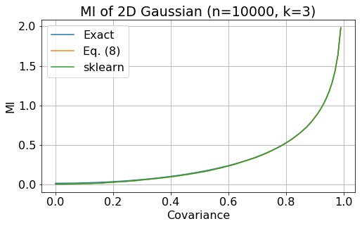
\[I(X, Y) = -\frac{1}{2} \log(\text{det}\sigma) \,. \label{eq:exact}\]

In the following plot, we show mutual information as a function of covariance. The blue line is the exact calculation using Eq. (\ref{eq:exact}), the orange line is the mutual information estimate calculated with Eq. (\ref{eq:8}), while the reen line is the mutual information calculation implemented in sklearn. The plot shows that the estimate is in agreement with the exact value.

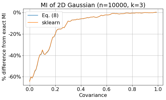
In the next plot, we show the percentage different between the mutual information estimate and the exact value Eq. (\ref{eq:exact}),

\[\frac{I_\text{estimate} - I_\text{exact}}{I_\text{exact}} \,.\]

The blue line is the difference between Eq. (\ref{eq:8}) and the exact value, while the orange line is the difference between sklearn calculation and the exact value. The plot shows that the error of the estimate decreases as the covariance of the data increases. However, the error can be rather big. Notice that the paper only shows the difference, not the percentage difference. When the value of MI is very small, a small difference can be translated to a big percentage difference. My calculation is slightly different from sklearn calculation because in sklearn, a small amount of noise is added to x see here.

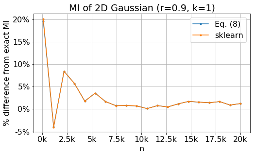
The next plot shows the percentage difference between mutual information estimate and the exact value for as a function of number of data points. The blue line is the exact value, the orange line is my calculation, while the green line is sklearn calculation. This plot shows that the error of the estimates decreases as the number of points increases. However for $n\gtrsim7500$, the error seems to dominated by systematic error.

Conclusion

From the above plots, we can see that we should take the estimate with a grain of salt. The statistics error can be large when the number of data points is small. In addition, if correlation between the data is very small, the percentage error of the estimate can be large. Furthermore, the above plot is based on normal distributed data, which the exact mutual information is known. For other distribution, please refer to the original paper for more information.

I wasn’t able to reproduce correct mutual information estimate based on the second formulation, Eq. (\ref{eq:9}). Please let me raise an issue if you see any mistakes in my calculation.

I do not really get the generalization of $H(X)$ to multi-dimension. However, the result of this paper is mainly empirical. So, I will let somebody else to worry about this. Perhaps by figuring this part out, one might be able to show why this estimates always give zero for variables that are not correlated.