[WIP] Learning Classifiers from Only Positive and Unlabeled Data
Learning Classifiers from Only Positive and Unlabeled Data
This post is based on Charles Elkan and Keith Noto. 2008. Learning classifiers from only positive and unlabeled data. In Proceedings of the 14th ACM SIGKDD international conference on Knowledge discovery and data mining (KDD ‘08). ACM, New York, NY, USA, 213-220. DOI: https://doi.org/10.1145/1401890.1401920
Positive and unlabeled (PU) learning is a problem where only positive and unlabeled examples are available. Unlike traditional data, unlabeled data contains both positive and negative examples. PU learning has many practical application. For example, in fraud related problems, one usually have the fraud examples and unlabeled examples typically contains both non-fraud examples and fraud examples that are not yet identified.
Results
The authors found that by assuming that for binary classification problem, if the positive examples are selected at random from the entire positive population, then the problem can be simplified to
- classical binary classification problem shifted by a constant factor, or
- traditional classification with different weight on the unlabeled examples. However, it is important to note that this assumption is not always true.
Setup
Let $x$ be an example and $y={0, 1}$ be the target. This is a classic binary classification problem and our model is
\[f(x)=p(y=1|x) \,.\]We call this traditional classifier.
In PU data, instead of having $y={0, 1}$, we have $s={0, 1}$ where $S\subset Y$. That is $p(y=1|s=1)=1$ and $p(y=0|s=1)=0$ but $p(y=0|s=0)\neq1$. We call $s=1$ is the positive set while $s=0$ is the unlabeled set. However, the goal of the problem is still trying to predict $y$, not $s$. Let the model that is trained on the PU data be
\[g(x) = p(s=1|x) \,.\]The goal is to find ways to relate $f(x)$ to $g(x)$. We call $g(x)$ a nontraditional classifier.
To make progress towards this goal, the author assumes that the positive samples are chosen complete at random, that is
\[p(s=1|x, y=1) = p(s=1|y=1) \,.\]The main result of this paper is
\[f(x) = g(x) / c \,,\]where $c=p(s=1|y=1)$.
Proof:
\begin{align} g(x) &= p(s=1|x) \nonumber \\ &= p(y=1,s=1|x) \nonumber \\ &= p(y=1|x)p(s=1|y=1,x) \nonumber \\ &= f(x)p(s=1|y=1) \,. \end{align}
Notice that this result depends on the assumption above, which is not always true.
Consequences of this results:
- If one only interested in rank ordering, then one can use $g(x)$ directly.
- $f(x)$ is a proper probability function if and only if $g(x) \leq p(y=1|s=1)$.
PU Learning as a Constant Shift of Traditional Binary Classifier
To estimate $c$, the approach that the author recommends is by using a validation set. Let $P$ be the validation set and $V$ be the labeled data in the validation set. Notice that for $x\in P$,
\begin{align} g(x) &= p(s=1|x) \nonumber \\ &= p(s=1|x,y=1)p(y=1|x) + p(s=1|x,y=0)p(y=0|x) \nonumber \\ &= p(s=1|x,y=1) \nonumber \\ &= p(s=1|y=1) \end{align}
Hence, an estimate of $c$ is
\[\hat c = \frac{1}{n}\sum_{x\in P}g(x) \,,\]where $n$ the cardinality of $P$.
PU Learning by Weighing Unlabeled Examples
Let $h(x,y)$ be any functions that we are interested to estimate. The expectation of $h(x,y)$ is
\begin{align} \mathbb{E}_{p(x,y,s)}[h(x,y)] &= \int_{x,y,s} h(x,y)p(x,y,s) \nonumber \\ &= \int_x p(x)\sum_{s=0}^1p(s|x)\sum_{y=0}^1p(y|x,s)h(x,y) \nonumber \\ &= \int_x p(x)\left(p(s=1|x)h(x,1)+p(s=0|x)\sum_{y=1}^1p(y|x,s=1)h(x,y)\right) \,. \end{align}
Notice that
\begin{align} \omega(x) \equiv p(y=1|x,s=0) &= \frac{p(s=0|x,y=1)p(y=1|x)}{p(s=0|x)} \nonumber \\ &= \frac{[1-p(s=1|x,y=1)]p(y=1|x)}{1-p(s=1|x)} \nonumber \\ &= \frac{1-c}{c}\frac{p(y=1|x)}{1-p(s=1|x)} \end{align}
Hence, an estimate of the expectation becomes
\[\hat{\mathbb{E}[h]} = \frac{1}{m}\left(\sum_{x,s=1}g(x)h(x,1)+\sum_{x,s=0}[1-g(x)]\omega(x)h(x,1)+[1-g(x)][1-\omega(x)]h(x,0)\right) \,,\]where $m$ is the cardinality of $X$.
To get an estimate for $y$, let $h(x,y)=y$, we have
\[\hat{\mathbb{E}[y]} = \frac{1}{m}\left(\sum_{x,s=1}g(x)+\sum_{x,s=0}[1-g(x)]\omega(x)\right) \,.\]Notice that the result that I derived here is not in agreement with the paper.
Application to Synthetic Data
In this Section, I applied the above result to some synthetic data I that generated. Notebook to produce these plots are at here
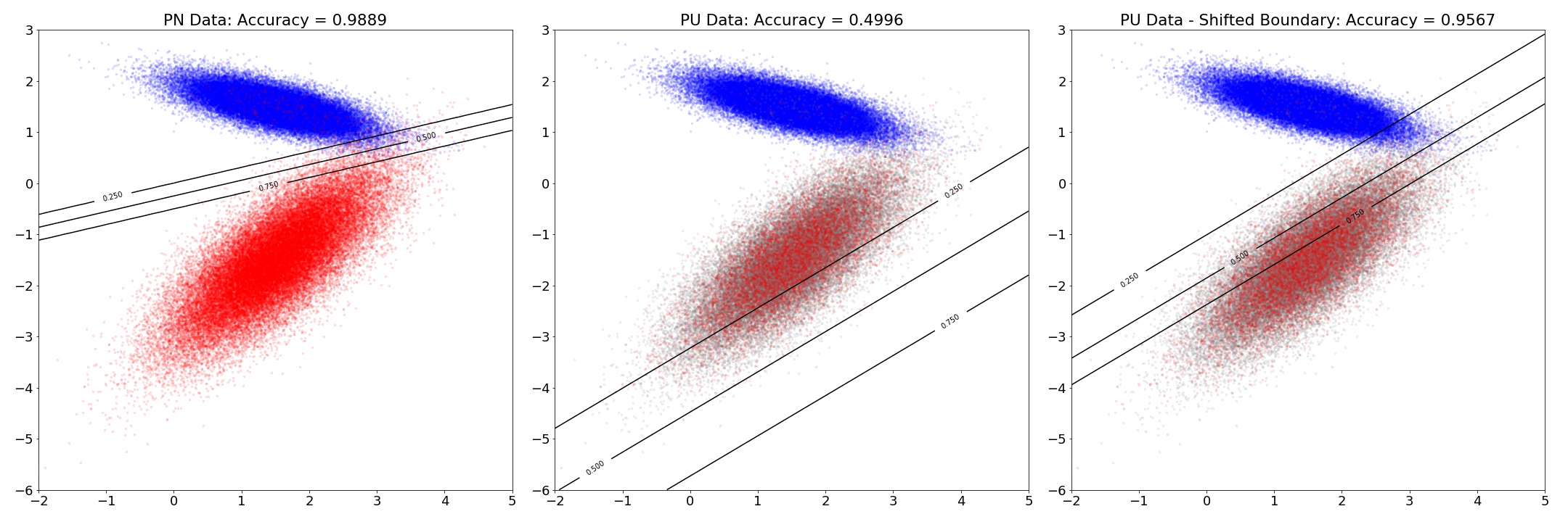
Visualizing Shift in Boundary
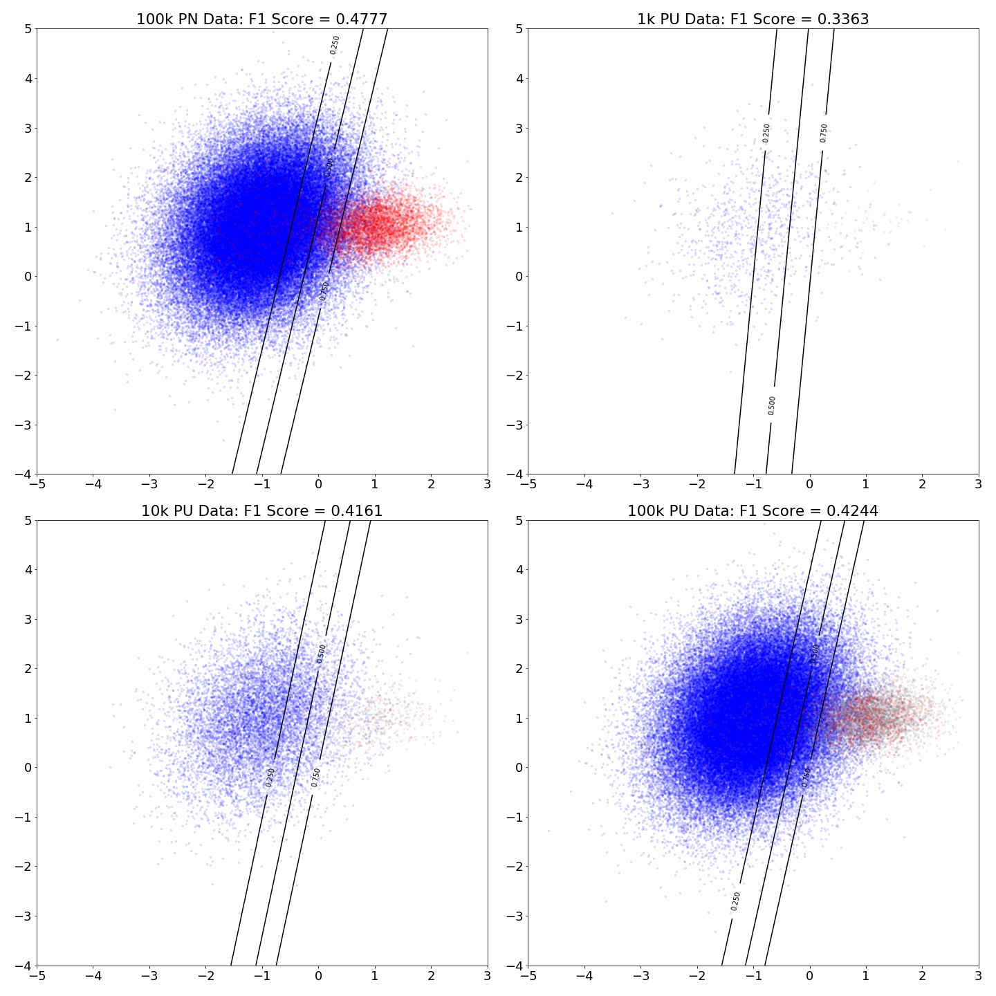
In this plot, I have 100k data with balanced class. This plot shows the shift in the decision boundary by applying (4).
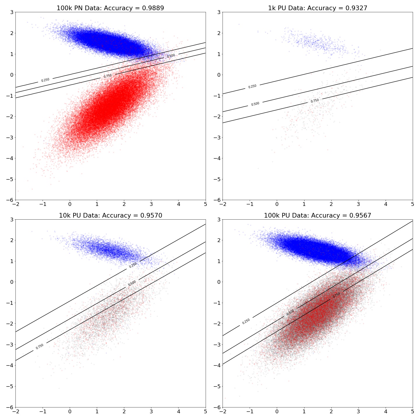
Dependence of the Accuracy on the Size of Dataset
This plot shows that as the accuracy improves as the available data increases. However, the accuracy stops improving after some threshold.
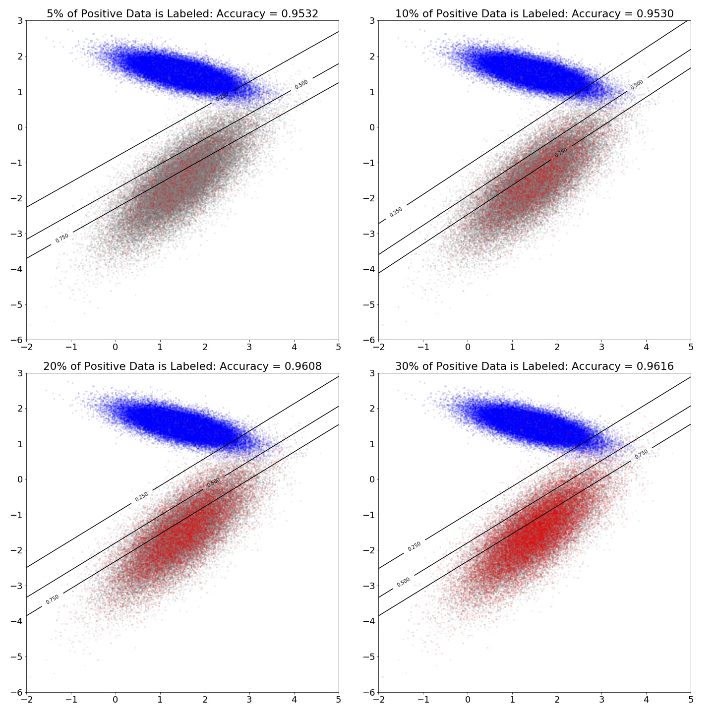
Dependence of the Accuracy on PU Ratio
This plot, as expected, shows the more positive data we have, the higher the accuracy of the classifier.
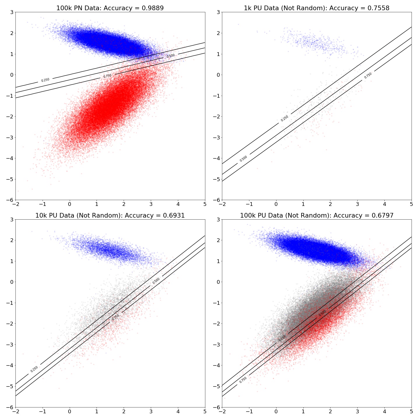
Imbalance Data
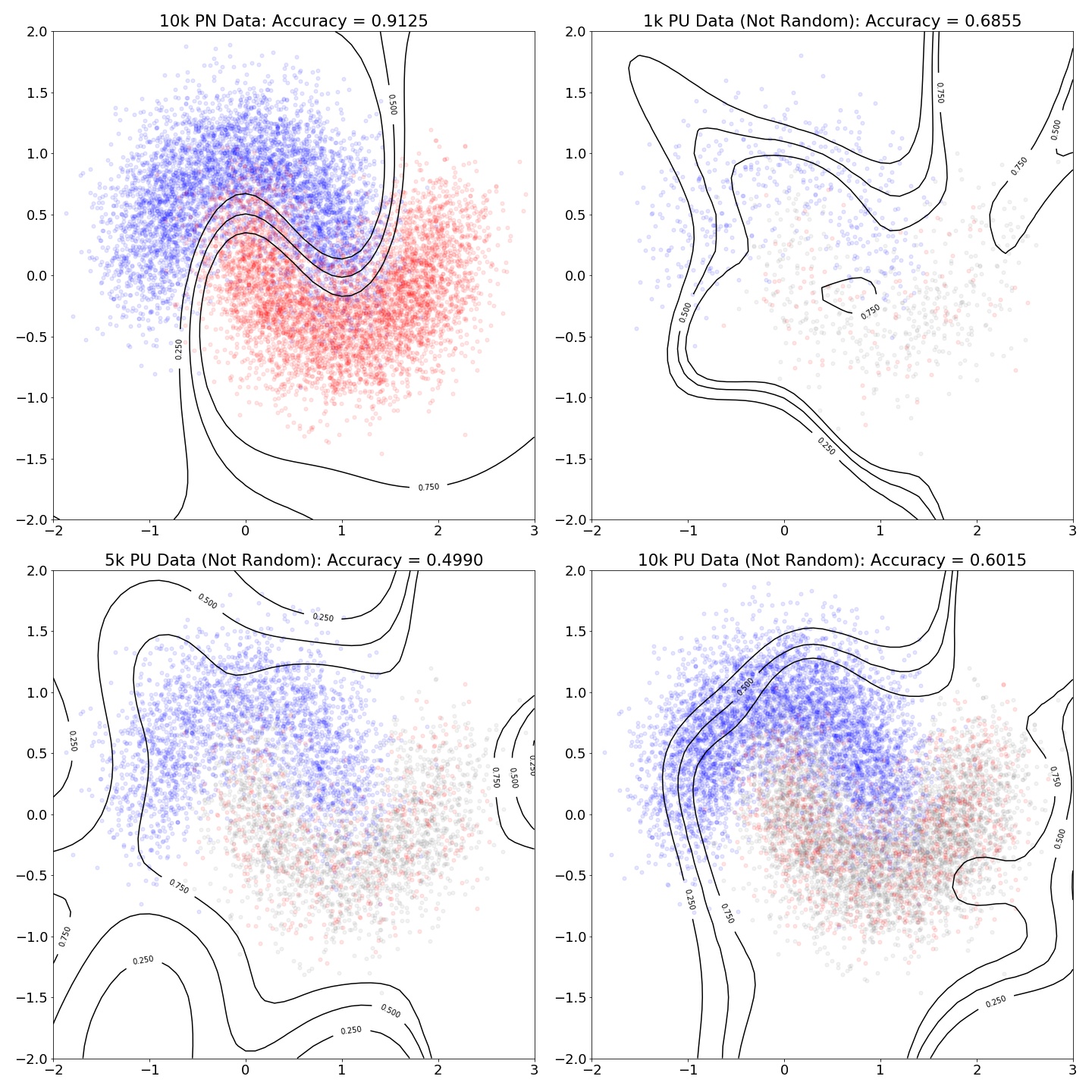
Unlabeled not at Random
Non-linear Boundary